Metrics in software observability

Metrics are used in a variety of domains, not just software. However I am a software developer: so in this article we’ll focus on some considerations worth keeping in mind when metrics are used for software observability, specifically timeseries metrics, with a deep dive in the Prometheus modelling for different types of metrics.

Let’s jump to a definition, how can we define a metric?

A metric is an aggregated measurement taken at a given point in time, sampled at regular interval.

As you can notice, we higlighted the two most important properites of metrics in observavility that we should always keep in mind when working with them.

Metrics are an aggregated measurement

When dealing with metrics, we have to remember that we’re dealing with aggregations. This has the nice effect of making the volume of generated data independent of the volume that is input to the system, making its estimates more reliable, however it does entail data loss. When looking at metrics only it might not be possible to investigate sparse issues and failures that do not affect the general trend.

Let’s make up one example where we record information about average served request latency: it doesn’t matter how many requests we serve (say 4), we output always one data point (the average in this case).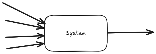

.

While we said that the amount of data is independent of the system input volume we must be mindful that the amount of generated data is directly proportional to the number of instances running. In the given example, if the 4 requests are spread across two instances of our system, we will generate 2 data points (the average of each instance).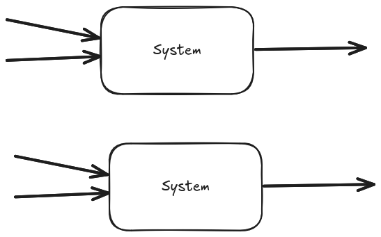

Metrics are taken at a given point in time

When looking at metrics, we must not make any assumption about what was happening between measurement intervals! That’s because metrics give us only the information available at the given point in time where the measurement is taken. Let’s use another example, and let’s take these two very different signals green and blue we want to measure.

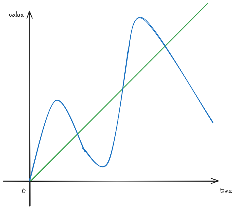
And let’s assume we record their values every 2 seconds.

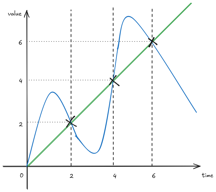
The resulting information available looks like the following.

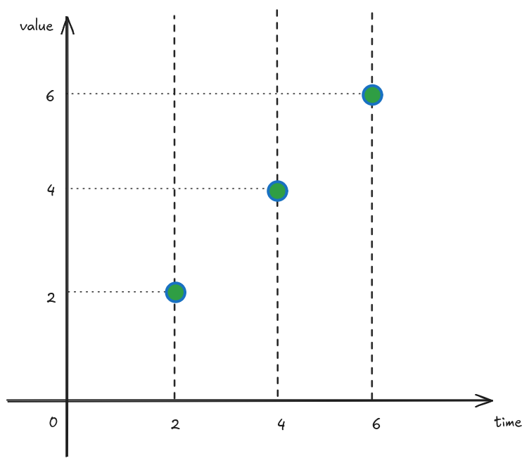
Given our information the two signals look identical, however we know they were originally wildly different! They just happened to briefly be the same when the measurements were taken. While this might be unlikely to happen, it does prove the point that we should not make assumption about anything that happened between measurements.

Prometheus metric types

Prometheus has been the de-facto standard monitoring tool for metrics for a long time. It’s beneficial to take a closer look to its foundational metric types to better understand how to effectively use them.

Counters

Counters represent monotonically increasing values. Usually these are used to measure things for which we don’t care about their absolute value, but rather how they change in time. For example, we might represent with a counter the number of requests served by our system: while it might be of litlte interest how many requests we served since startup, it’s interesting to see increase in traffic compared to before. To visualise the change in a counter metric, we should look at the rate function.

What is the result of the rate function

That has been a question it took my a while to answer when first getting started with Prometheus. What helped my understanding better the rate function was writing down the mathematical formula for it. Given a counter c, the rate function of c over time period T is:

$$ rate_t(c, T) = \frac{c(t) - c(t - T)}{T} $$

So we take the value of counter c at the current time t, subtract is value T seconds before, and divide by T. If you have a mathematical eye, you might notice that for values of T that tend to 0, the rate funciton is the first degree derivative of the coutner! And since the counter is monotonically increasing, we can be sure that the rate funciton will never be negative. Another thing we can deduce from this, is that when the rate is 0 the counter funciton is constant. So the unit of measure of the result of the rate function is the unit of measure of the original signal per second. In our counter example, the unit of measurement of the original signal was number of requests so the result of the expression sum(rate{http_server_requests_seconds_count}[5m])) would be in requests per seconds or more succintly req/s.

Gauges

Gauges on the other hand represent values that can either increase or decrease. A typical example of something to measure with a gauge would be memory usage, or number of elements in a work queue.

If you are measuring number of elements in a work queue, remember to not make any assumptions on what happens between measurements! If a work element is added and consumed between 2 consecutive measurement intervals, it might look like no work has been done.

It’s best to not use the rate function with gauges since its implementation relies on the fact that counters are monotonically increasing to detect counter resets.

Histograms

Histograms are useful when we want to measure the distribution of our data. For example, just looking at the averge of our response time might not be enough, we want to be able to see the distribution of response times to build SLO based alerts. Histograms represent data divided into buckets, where each bucket is a counter. For example, we might record how many requests we served in under 50ms, how many between 50 and 100ms, between 100 and 500ms, between 500ms and 1s and in more than 1s.

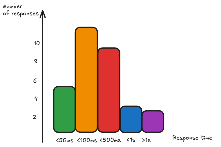
This way we can see how many we served unders our SLO target. Given the fact that the bucket measurements are counters, we can also aggregate between histograms generated by different instances.

Summaries

Summaries are similar to histograms in the sense that they represent a distribution, however instead of reporting the raw counters they report the quantiles computed client side. This effectively makes aggregations server side not mathematically sounds, so use summaries only when you know you won’t need to aggregate your measurements across instances.

Recap

Metrics come in handy when we want to observe our system large scale trends: this use case is particularly well suited for alerting purposes, to know when something goes wrong more than why. For the latter purposes, logs and traces are better suited to complete the picture. The aggregated nature of the collected data makes it also affordable to store for longer period of time, so metrics can be used to track and analyze historical behaviours.

A more in depth discussion about effective alerting can be found at SLO practice with SpringBoot and Prometheus.